Proc Tabulate Gallery with over 30 SAS Examples
Below are the SAS examples from the A to Z Analysis and Validaton using Proc Tabulate e-Guide.
Select from on of the table layouts below. Select the 'SAS Code' link below each table layout to copy and paste the SAS example. Next, customize the working Proc Tabulate syntax version as needed. One dimensional tables - 1a, and 1b. Two dimensional tables - 2, 3, 4, 5, 6a-g, 7a-b, 8, 10, 11, 12, 13, 14, and 15a-b. Three dimensional tables - 9.
See also Proc Report Gallery. Return to Proc Tabulate.
Proc Tabulate Default Settings: Column Structure, Horizontal Additions, Formatted Display Order, N for categorical data and SUM for continuous data, No %, Non-missing data displayed, and No Subtotals/Totals
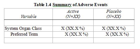
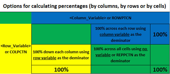
Percentage Calculations: Make sure the denominator is correct by first deleting duplicate records. Before calculating percentages of subjects with AEs by System Organ Class and Preferred Term, for example, make sure to PROC SORT with NODUPKEY option and BY _ALL_ in advance. For percentages of subject with AEs by System Organ Class, for example, apply NODUPKEY with BY USUBJID AEBODSYS.
- Formatted_order_categorical_and_continuous_data_as_columns
- Formatted_order_categorical_and_continuous_data_as_rows
- Formatted_order_categorical_data_100_by_column
- Frequency_order_categorical_data_100_by_column
- Data_order_categorical_data_100_by_column
- Data_order_categorical_data_100_by_row
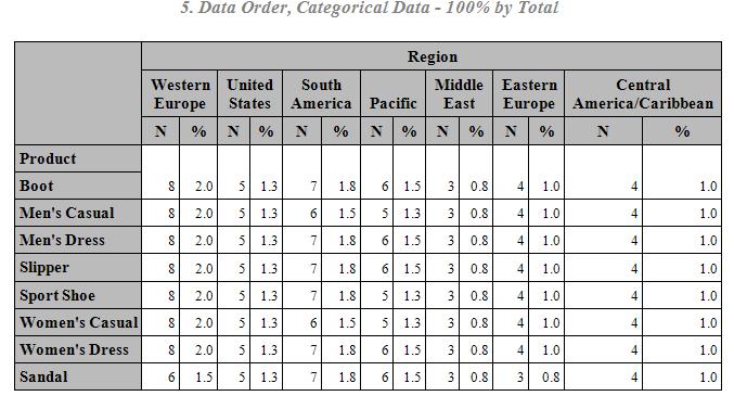
- Data_order_categorical_data_100_by_total
- Data_order_categorical_data_100_by_total
- Mixing_categorical_and_continuous_data_percentages
- Multiple_label_continuous_data_percentages
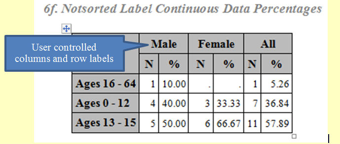
- Notsorted_label_continuous_data_percentages
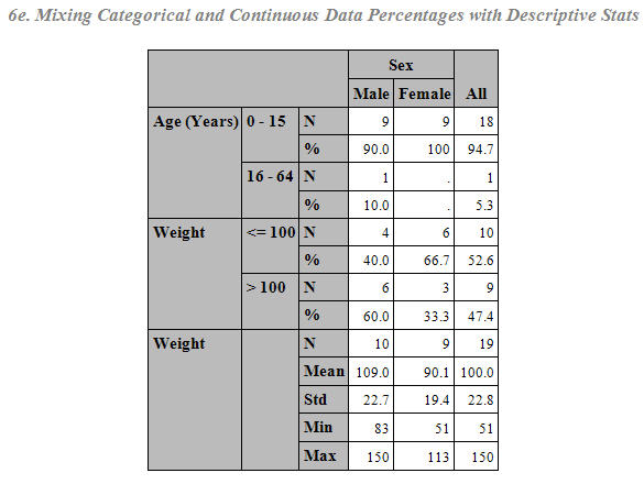
- Mixing_categorical_and_continuous_data_percentages_with_descriptive_stats
- Notsorted_Label_Continuous_Data_Percentages
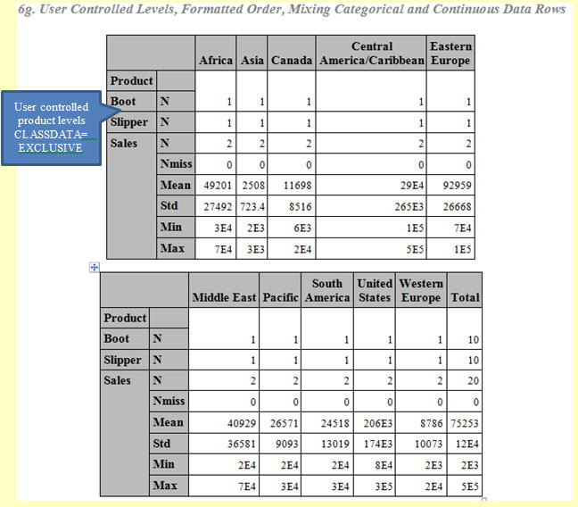
- User_Controlled_Levels_Formatted_Order_Mixing_Categorical_and_Continuous_Data_Rows
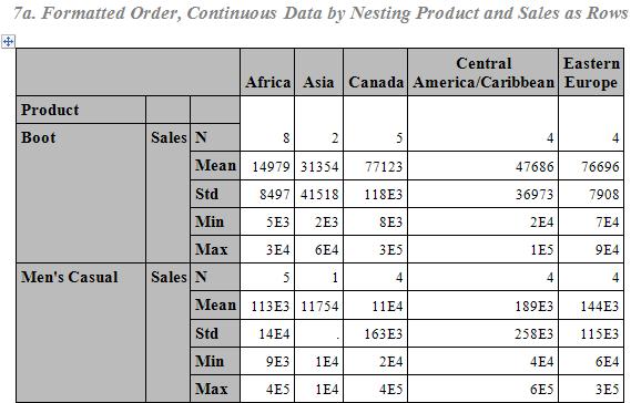
- Formatted_order_continuous_data_by_nesting_product_and_sales_as_rows
- Formatted_order_continuous_data_by_nesting_product_and_sales_as_columns
- Formatted_order_continuous_data_by_product
- Formatted_order_continuous_data_by_product_page
- Formatted_order_continous_data_by_nesting_by_region_and_subsidiary
- Product_distribution_by_nesting_by_region_and_subsidiary
- Product_distribution_by_nesting_by_region_and_subsidiary_with_subtotals
- Formatted_order_multiple_continuous_row_data
- Analysis_of_categorical_data_by_column_row_and_table
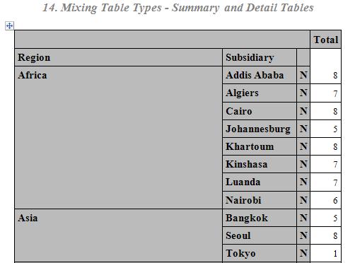
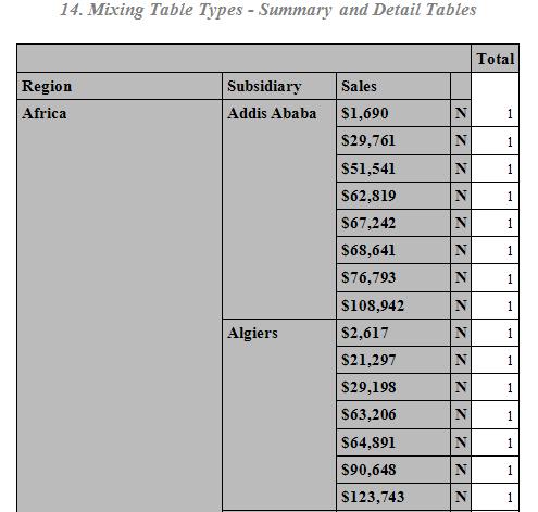
- Mixing_table_types_summary_and_detail_tables
- Single_Column_Descriptive_Stats_as_Rows
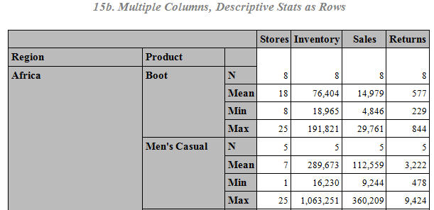
- Multiple_Columns_Descriptive_Stats_as_Rows
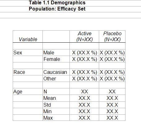
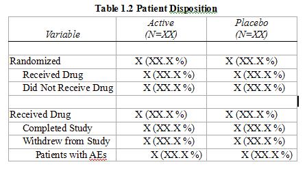
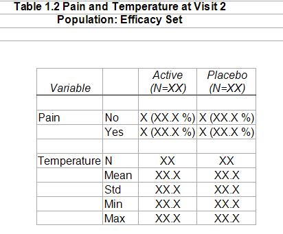
- Pharmaceutical_Table_Examples

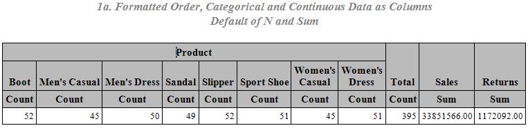
1a. Formatted order, categorical and continuous data as columns
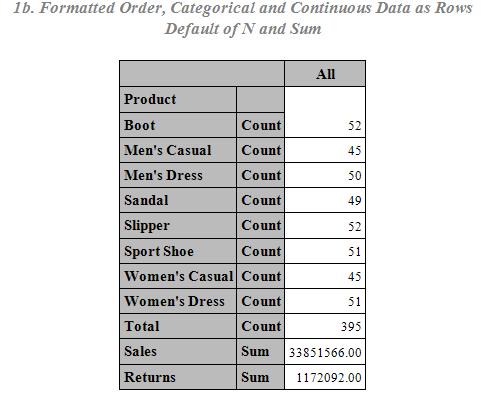
1b. Formatted order, categorical and continuous data as rows
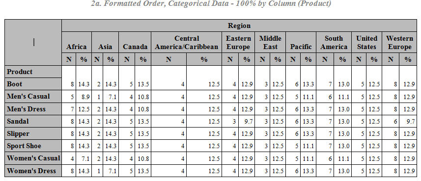
2a. Formatted order, categorical data - 100% by column
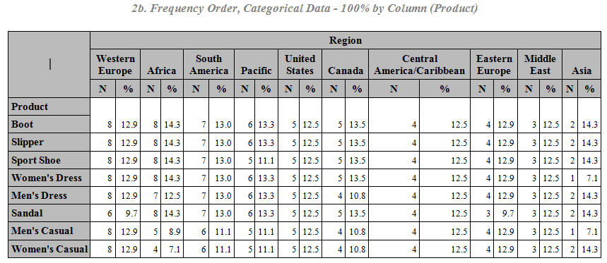
2b. Frequency order, categorical data - 100% by column
3. Data order, categorical data - 100% by column

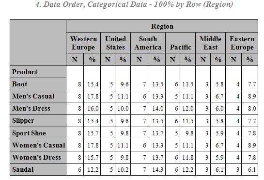
4. Data order, categorical data - 100% by row
5. Data order, categorical data - 100% by total
6a. Formatted order, mixing categorical and continuous data rows
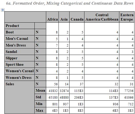
(SAS Code) (Pharmaceutical Example)
6b. Mixing categorical and continuous data percentages

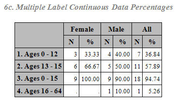
6c. Multiple label continuous data percentages
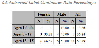
6d. Notsorted label continuous data percentages
6e. Mixing categorical and continuous data percentages with descriptive stats
6f. Notsorted Label Continuous Data Percentages
6g. User Controlled Levels, Formatted Order, Mixing Categorical and Continuous Data Rows
7a. Formatted order, continuous data by nesting product and sales as rows
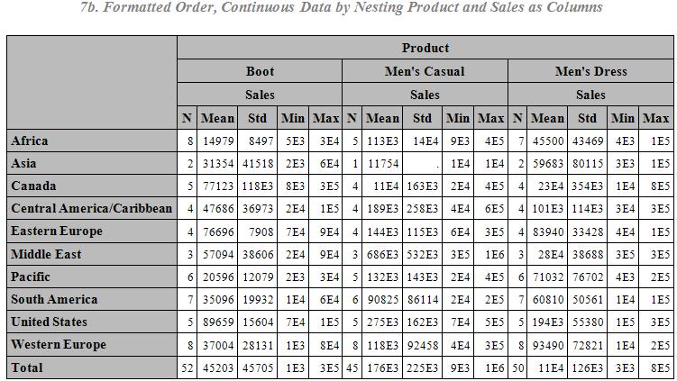
7b. Formatted order, continuous data by nesting product and sales as columns
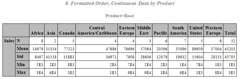
8. Formatted order, continuous data by product
9. Formatted order, continuous data by product page

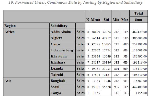
10. Formatted order, continous data by nesting by region and subsidiary
11a. Product distribution by nesting by region and subsidiary

11b. Product distribution by nesting by region and subsidiary with subtotals

* Example of a three level hierarchy with subtotals;
proc tabulate data=studylib.adae missing;
class trt01a usubjid aebodsys aedecod aetoxgr;
* Levels 1 ( 2a SUM) ( 2b SUM) ( 3 SUM);
table aebodsys*(aetoxgr all aedecod all aedecod*aetoxgr all)
, (trt01a)*(n='N'*f=5.0);
where SAFFL='Y';
run;
12. Formatted order, multiple continuous row data

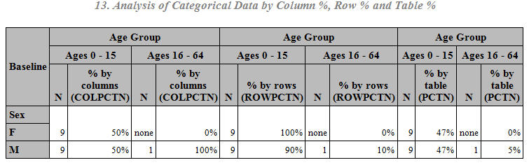
13. Analysis of categorical data by column %, row % and table %
14. Mixing table types - summary and detail tables
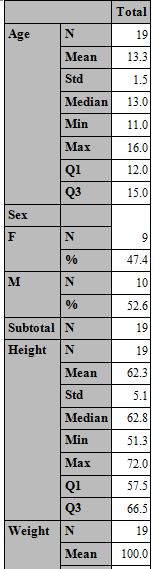
15a. Single Column, Descriptive Stats as Rows

15b. Multiple Columns, Descriptive Stats as Rows
Pharmaceutical Table Examples (Production tables to validate. Not produced by Proc Tabulate)